Views

Views are attribute visualisations. Every type of attribute supported by Aguila has a default view type which will be shown when no view is explicitly selected when starting up Aguila. For example, a raster attribute will be shown in the map view and a time series in a time graph view. Some attribute types can be shown in multiple view types. A spatio-temporal raster attribute can be shown in a map view and a time graph view at the same time, for example.

Aguila uses the notion of a cursor to enable the views to decide which part of an attribute data set to visualise. The cursor consists of a set of coordinates that the user can set, like the current time step and the current spatial x- and y-coordinates. The current time step determines which map of a spatio-temporal attribute is shown, for example. And the current spatial coordinate determines for which spatial location of a spatio-temporal attribute the time graph is shown.

Views enable the user to change the cursor. For example, in a map view, the spatial coordinates of the cursor can be changed by clicking in the map. And in a time graph view, the time coordinate of the cursor can be changed by clicking in the graph. All views will respond to a change of the cursor. See section Cursor And Values View for a view for viewing and changing the current cursor coordinates.

Apart from the cursor there are more global properties used by Aguila to maintain links between the views. Examples of those are the scale of a map and the pan position. Because of this, all map views will always show the same area.

Attributes have draw properties, for example the palette used to select colours used to visualise the attribute. These properties are shared among the views, so each attribute always uses the same properties, no matter in how many views the attribute is shown. Changing the properties of the attribute in one view, also changes the properties of the attribute in the other view(s).

All views have a similar layout. The largest part is taken up by the visualisation itself, and on the left there is a legend for each attribute visualised. Between the legend and the main visualisation there is a splitter which can be dragged to make the legend larger or smaller relative to the main visualisation. At the top there are a menu bar and a toolbar.

Right-clicking the legend of an attribute brings up a context menu with actions specific for the selected attribute. Some actions are always available and some actions are available depending on the characteristics of the selected attribute. For example, the action to show an attribute in a time graph view is only available for a temporal attribute.

Here is a list of common attribute context menu actions:

Attribute context menu actions

Menu item	Effect
Edit draw properties	Shows the Draw Properties dialog, see section Draw Properties Dialog.

Double-clicking the attribute legend shows the draw properties dialog also.

For spatio-temporal attributes, the attribute context menu has a Show Time Series action. This will show the attribute in a new, linked, time graph view.

Cursor And Values View

All attributes shown by Aguila are put in the cursor and values view too. This view is normally not visible when the application starts (unless requested with the valueOnly program option (see section Program options).

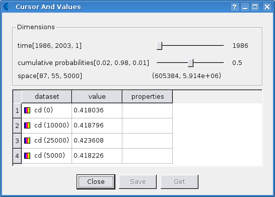
This view shows the current global cursor coordinates and the attribute values at the current cursor position.

The view consists of an upper part with the current cursor coordinates and a lower part with the values of all attributes loaded. The cursor sliders allows navigating through the dimensions such as time and space (see section Dimensions). Each slider has a knob for the current position.

Cursor slider actions

Change position	Slider action
Set slider one position backwards	Click on the slider part left from the knob
Set slider one position forward	Click on the slider part right from the knob
Set slider to specific position	Drag knob to position

In the value list at the bottom the data names and their values at the current cursor position are shown.

If Aguila started with the cursorValueMonitorFile program option, the Save button is enabled to append the current data in that file.

If Aguila started with the fileToGetCursorValue program option, the Get button is enabled to set the coordinate dimensions to that file contents.

Map view

A map view shows spatial attributes by a map. This map visualises the spatial variation of the attribute, given the current cursor position.

Map Controls

Map controls.

Effect	Control
change spatial cursor	left mouse click
pan	left mouse drag
continuously change spatial cursor (prevents panning)	Ctrl+left mouse drag
move map to the right	h / left mouse drag right
move map to the left	l / left mouse drag left
move map to the bottom	k / left mouse drag down
move map to the top	j / left mouse drag up
zoom in	Ctrl+k / left mouse double click / scroll mouse
zoom out	forward Ctrl+j / scroll mouse backward
Zoom by rectangle	Shift+left mouse drag
reset	r

Time Graph View

A time graph view shows temporal attributes by a single line. This line visualises the temporal variation of the attribute, given the current cursor position. The current time can be changed by clicking or dragging in the graph.

The attribute context menu has a Save graph data as... action. This enables one to export the data of a single graph line.

Drape View

The drape view shows a scalar spatial raster attribute as a surface (or sheet) which floats in space. Additional spatial raster attributes can be shown on top of this surface.

You can change some properties of the drape view by right clicking your mouse in the map view (the one which shows the sheet) and selecting Properties. The properties dialogue for the map view will be shown.

Note

The drape view can only be used when Aguila was built with OpenGL support.

Drape Controls

There’s a difference between controlling the camera (‘your head’) and the 3D scene. You can control the position and aim of the camera (see the table below). You can only control the orientation of the scene (see the second table below). Together these controls enable you to look at every part of the scene from everywhere.

Controls for changing the position and orientation of the camera.

Effect	Control
look left	h / left mouse drag left / right mouse drag left
look right	l / left mouse drag right / right mouse drag right
look up	k / right mouse drag forwards
look down	j / right mouse drag backwards
roll clockwise	n
roll counter-clockwise	m
move left	Shift+h / left-right mouse drag left
move right	Shift+l / left-right mouse drag left
move up	Shift+k / left-right mouse drag forwards
move down	Shift+j / left-right mouse drag backwards
move forward	Shift+Up / Ctrl+k / left mouse drag forwards
move backwards	Shift+Down / Ctrl+j / left mouse drag backwards
reset	r

Controls for changing the orientation of the scene.

Effect	Control
rotate clockwise around z-axis	Left
rotate counter-clockwise around z-axis	Right
rotate clockwise around x-axis	Up
rotate counter-clockwise around x-axis	Down
reset	r

The camera and the scene have their own coordinate system which can be moved and rotated independently from each other. You should interpret the above controls relative to the direction of the coordinate system of the camera or the scene. For example, moving the camera forward means moving the camera in the direction of the camera. This might be in a direction away from the scene!

Camera’s

Apart from the camera whose position and orientation can be changed, there are 5 more camera’s in the scene. These static camera’s are positioned in such a way that it is possible to see the relative position of the scene and the mobile camera. The table below gives a list of camera’s you can choose from (note the correspondence between the shortcuts and the layout of the numeric keypad on your keyboard).

Camera’s.

Camera	Shortcut
Top	5
Front	2
Left	4
Back	8
Right	6
Mobile	0

Shortcuts

Shortcuts.

Effect	Shortcut
exaggerate heights	Plus (+)
understate heights	Minus (-)
enlarge quad length	Shift+q
decrease quad length	q

2D Multimap View

2D Multimap mode can be enabled when multiple scenarios are provided, that need to be compared side by side. Without duplication of window borders, legends, etc., in this mode, multiple maps are organized in panels over a regular lattice, and shown in a single window. Zoom/pan/identify actions, as well as legend modifications are now reflected automatically over all panels.

Aguila does not provide interactive setting of the panel layout; it needs to be set on the command line or in the configuration file specified on startup. If it is not specified, all maps (scenarios) will be shown in different windows, and e.g. legend changes will only reflect to the window at which it is applied.

Probability Graph View

Aguila can show probability distribution functions (cumulative probabilities and exceedance probabilities) for continuous random variables. The probability graph view is available only when the data are specified as a probability distribution, using a set of quantiles (see section Data set types).

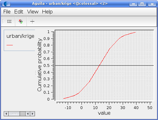
For uncertain attributes, the attribute context menu has a Show Probability Plot action. This will show the attribute in a new, linked, probability graph view. This view shows, for the current location and time step, the distribution function for the data, or the set of distribution functions for the set of scenarios.

The view shows a horizontal line at distribution value 0.5, indicating that the map currently shows the median value. The horizontal line can be dragged to show other quantile values in the map view or time plot.

As an alternative view, the distribution function values for a given threshold value (one minus the exceedance probability) can be shown by pressing the tool button with the + symbol, or through menu items View | Toggle Marker. This will flip the horizontal line into vertical position, allowing modification of the threshold (attribute) value for which distribution function values (probabilities) will be shown.

Pressing the + tool button again returns to quantile views.

Dragging the line may, for larger data sets, be slower in vertical mode than in horizontal mode. The reason is that in vertical mode, besides a linear interpolation, a lookup needs to take place, because the function is specified for a known set of (constant) probability values, and not as probabilities for a known set of attribute (data) values.